From Dice to Agents: Reinforcement Learning in One Set of Symbols
Most introductions to reinforcement learning for language models start in the middle, with PPO or GRPO already on the table. This post starts from a dice game instead and adds one idea at a time until we arrive at the RL used to train LLMs and agents today.
Here is the route:
- p and f: what an expectation is.
- Monte Carlo: estimating an expectation by sampling.
- q: sampling from the “wrong” distribution and correcting for it.
- The basic pieces of RL: states, actions, policies, rewards.
- Policy gradients and baselines: how to actually improve a policy.
- PPO: how to reuse data safely.
- LLM RL: putting a language model into the picture.
- Agentic RL: letting the model use tools over many turns.
You only need a little probability (what “the probability of \(x\)” means) and a rough idea of what a gradient is. Everything else is built up as we go. If you keep reading to the end, I hope PPO’s clip, GRPO’s group average, and the corrections people add in modern LLM training will stop looking like a pile of tricks. They are all answers to the same two questions, which we will meet in Section 2.
1. p and f: what an expectation actually computes
Let’s play a game. You roll a die, see the number \(x\), and I pay you \(x^2\) dollars. Roll a 3, get 9 dollars. Roll a 6, get 36. How much do you win per game, on average?
To answer this we need two ingredients:
- \(p(x)\) is the probability of each outcome. Think of it as the rule the world uses to produce \(x\). For a fair die, every face has \(p(x) = 1/6\).
- \(f(x)\) is the quantity you care about. It gives each outcome a score. Here \(f(x) = x^2\).
Combine them and you get the expectation, a probability-weighted average of the score:
\[\mathbb{E}_{x\sim p}[f(x)] = \sum_x p(x)f(x)\]The notation \(x \sim p\) just means “\(x\) is drawn from \(p\)”. For our die:
\[\frac{1+4+9+16+25+36}{6} \approx 15.17 \text{ dollars.}\]That’s it. Hold on to these two letters: \(p\) says how likely each outcome is, and \(f\) says how good it is. The rest of the post keeps reusing them.
2. Monte Carlo: when you can’t add everything up, try it
A die has six outcomes, so we could just add them up. But what if \(x\) is “a 1,000-token answer written by a language model”? With a vocabulary of about 100,000 tokens, there are \(100{,}000^{1000}\) possible answers. No computer will ever add up that many terms.
The Monte Carlo method does the obvious thing instead: actually play the game \(N\) times and average what you won.
\[\mathbb{E}_{p}[f] \approx \frac{1}{N}\sum_{i=1}^N f(x_i),\quad x_i \sim p\]You never have to list every outcome. You only need a way to draw outcomes.
How accurate is this? The error shrinks roughly like \(1/\sqrt{N}\), so four times as many samples cuts the error in half. The error also depends on how much \(f\) jumps around from sample to sample. This spread is called the variance. If the payout is usually nothing but occasionally a million dollars, you will need a huge number of rolls before your average settles down.
So Monte Carlo comes with two conditions, and they are the thread running through this whole post:
(1) You must be able to draw samples from \(p\). (2) The variance must not be too large.
Every technique from here on exists to deal with one of these two conditions.
3. q: when you can’t sample from the distribution you care about
Now a twist. You want the average payout of a loaded die, which we’ll call \(p\). You know how it’s loaded: a 6 comes up half the time, and each other face comes up 10% of the time. The catch is that you don’t have this die. The only die you can actually roll is a fair one, which we’ll call \(q\).
Can you still estimate the loaded die’s average? Yes. Roll the fair die, but give each result a weight of \(p(x)/q(x)\) before averaging:
\[\mathbb{E}_{p}[f] = \mathbb{E}_{q}\Big[\frac{p(x)}{q(x)}f(x)\Big]\]Why does this work? Look at a single roll of 6. On the loaded die it happens with probability 0.5; on the fair die, \(1/6\). So its weight is \(0.5 / (1/6) = 3\). In the world you care about, a 6 is three times as common as in the world you’re sampling from, so each 6 you see should count three times. Every other face gets weight \(0.1 / (1/6) = 0.6\), because those faces are rarer on the loaded die. This trick is called importance sampling.
A few lines of code show it working:
import numpy as np

rng = np.random.default_rng(0)
faces = np.arange(1, 7)
f = faces ** 2
p = np.array([0.1] * 5 + [0.5])  # loaded die: the distribution we care about
q = np.full(6, 1 / 6)            # fair die: the one we can actually roll

x = rng.choice(faces, size=100_000, p=q)
w = p[x - 1] / q[x - 1]          # importance weights

print(f[x - 1].mean())           # ≈ 15.17, the fair die's average
print((w * f[x - 1]).mean())     # ≈ 23.5, the loaded die's average
The exact answer for the loaded die is \(0.1 \times (1+4+9+16+25) + 0.5 \times 36 = 23.5\), and the weighted estimate lands right on it.
There is a catch, and it matters a lot later. If \(p\) and \(q\) are very different, some samples will get enormous weights. Imagine an outcome that \(q\) almost never produces but \(p\) produces often: when it finally shows up, its weight might be 1,000, and that single sample drowns out everything else. The variance explodes, which breaks condition (2) from Section 2.
Rule of thumb: importance sampling only works well when \(q\) is close to \(p\).
This one rule is the origin of PPO’s “clip”, which we’ll reach in Section 6.
4. The basic pieces of RL
So far each game was a single roll. Real problems are usually a sequence of decisions: a chess game, a robot walking, a model writing an answer one word at a time. Each decision changes the situation, and the payoff often only arrives at the end.
Background: what makes RL different. In supervised learning, someone tells the model the right answer for each input. In reinforcement learning, nobody does. The model tries things, gets a score, and has to work out for itself which choices led to the good scores. It’s learning by trial and error.
Here is the vocabulary:
- State \(s\): the current situation, such as the position of the pieces on a chessboard.
- Action \(a\): what you choose to do in that state.
- Policy \(\pi_\theta(a \mid s)\): the probability of choosing each action in a given state. This is the “player”. The \(\theta\) stands for its adjustable parameters, for example the weights of a neural network. Changing \(\theta\) changes how the player behaves.
- Reward \(r\): the score the environment gives you after an action. It is often zero until the very end.
- Trajectory \(\tau\): the full record of one game: \(s_0, a_0, r_0, s_1, a_1, r_1, \ldots\)
- Return \(R(\tau)\): the total score for the whole game.
The goal is to find the parameters \(\theta\) that make the average return as high as possible:
\[J(\theta) = \mathbb{E}_{\tau\sim\pi_\theta}[R(\tau)]\]Now compare this with Section 1. It’s the same shape:
- \(p\) is the probability of each trajectory when you play with the current policy.
- \(f\) is the return \(R(\tau)\).
So RL is just a Monte Carlo expectation problem. The one new thing is that \(p\) now contains the parameters we are trying to change.
One more word you will see everywhere: a rollout is simply playing one game with the current policy and recording the trajectory. In our language, a rollout is drawing one sample from \(p\).
5. Improving the policy: policy gradients and baselines
We want to increase \(J(\theta)\). The usual way to increase a function is to compute its gradient, the direction in which it goes up fastest, and take a small step that way. The difficulty is that \(\theta\) sits inside the probability \(p\), not inside \(f\), so it isn’t obvious how to differentiate.
Background: the log-derivative trick. One line of calculus gets us out of this. Since \(\nabla \log p = \nabla p / p\), we can write \(\nabla p = p \, \nabla \log p\). Plugging that in:
\[\nabla_\theta J = \sum_\tau \nabla_\theta\, p_\theta(\tau)\, R(\tau) = \sum_\tau p_\theta(\tau)\, \nabla_\theta \log p_\theta(\tau)\, R(\tau) = \mathbb{E}_{\tau \sim p_\theta}\big[\nabla_\theta \log p_\theta(\tau)\, R(\tau)\big]\]The gradient is itself an expectation under \(p\), so we can estimate it with Monte Carlo, i.e. with rollouts. Also, the probability of a trajectory is a product of the policy’s choices and the environment’s responses. The environment part doesn’t depend on \(\theta\), so only the policy’s log-probabilities survive the gradient.
Averaging over \(N\) rollouts gives the classic algorithm REINFORCE (Williams, 1992):
\[\nabla_\theta J \approx \frac{1}{N}\sum_{\text{rollouts}}\sum_t \nabla_\theta \log\pi_\theta(a_t \mid s_t)\cdot R\]It reads more simply than it looks:
- \(\nabla_\theta\log\pi_\theta(a \mid s)\) is the direction that makes this action more likely.
- \(R\) says how hard to push in that direction.
In plain words: play a game. If it went well, make the moves you made more likely. If it went badly, make them less likely.
The problem. Suppose every game scores somewhere between 90 and 100. Then \(R\) is always large and positive, so every action gets pushed up, some a bit more than others. The useful information, which games were better than the others, is hidden in small differences between big numbers. The estimate is very noisy, which is condition (2) failing again.
The fix: compare against a baseline. Subtract a reference value \(b\) and use
\[A = R - b\]in place of \(R\).
- Games that went better than usual get \(A > 0\) and their actions are pushed up.
- Games that went worse than usual get \(A < 0\) and their actions are pushed down.
- \(A\) is called the advantage. It answers the question “how much better did this go than usual?”
Surprisingly, this doesn’t bias the gradient at all. As long as \(b\) doesn’t depend on the action taken, its contribution averages out to zero, because the probabilities of all actions always add up to 1:
\[\mathbb{E}_{a\sim\pi}\big[\nabla_\theta\log\pi_\theta(a \mid s)\, b\big] = b\,\nabla_\theta \sum_a \pi_\theta(a \mid s) = b\,\nabla_\theta 1 = 0\]So we get the same average gradient with much less noise. That’s a free win.
Where does \(b\) come from? There are two common choices, and the difference between them becomes important when we get to LLMs:
- Learn a critic \(V(s)\). Train a second network to predict “starting from this state, what score do I usually get?” This setup is called actor-critic (the policy is the actor, and the value network is the critic), and it is the classic way PPO is used. You can push this further: instead of playing every game to the end, stop early and let \(V\) estimate the rest. This is called bootstrapping. It trades a little bias for a lot less variance (Schulman et al., 2015).
- Try the same starting point several times, and use the average score of those tries as \(b\). No extra network needed. This is the idea behind GRPO and RLOO, which we’ll see in Section 7.
6. Reusing data: q comes back, and we get PPO
Rollouts are expensive. For a language model, generating thousands of answers takes a lot of GPU time. So after collecting a batch, we’d like to take several update steps on it, not just one.
But notice what happens after the first step. The policy is now a new \(\pi_\theta\), while the data was produced by the old policy, \(\pi_{\text{old}}\). We want an expectation under one distribution, but our samples came from another. That’s exactly the loaded-die situation from Section 3:
- \(p = \pi_\theta\): the new policy, the one we care about.
- \(q = \pi_{\text{old}}\): the old policy, the one the data came from.
So, just like with the dice, we reweight each action by a ratio:
\[\rho_t = \frac{\pi_\theta(a_t \mid s_t)}{\pi_{\text{old}}(a_t \mid s_t)}\]And now the rule of thumb from Section 3 kicks in: this only works if \(q\) stays close to \(p\). If we take too many steps on the same data, the new policy wanders away from the old one, the ratios get extreme, and training becomes unstable.
PPO (Proximal Policy Optimization, Schulman et al., 2017) handles this by clipping the ratio to the range \([1-\epsilon, 1+\epsilon]\), with \(\epsilon\) usually set to 0.2:
\[L^{\text{clip}}(\theta) = \mathbb{E}_t\Big[\min\big(\rho_t A_t,\ \operatorname{clip}(\rho_t, 1-\epsilon, 1+\epsilon)\, A_t\big)\Big]\]The formula looks busy, but the behavior is simple:
- If an action was good (\(A > 0\)) and the new policy already makes it more than 20% more likely than before (\(\rho > 1.2\)), stop pushing it up.
- If an action was bad (\(A < 0\)) and the new policy already makes it more than 20% less likely (\(\rho < 0.8\)), stop pushing it down.
- Otherwise, update as usual.
In other words, each batch of data is allowed to move the policy only a limited distance. That keeps \(q\) close to \(p\) and keeps the variance under control.
A side note for the careful reader: strictly speaking, the importance weight for a whole trajectory is the product of the per-step ratios. PPO uses one ratio per step, which is only a good approximation when the two policies are close. That’s one more reason to keep them close.
7. LLM RL: putting a language model into the picture
Background: a language model is already a policy. A language model reads the text so far and outputs a probability for every possible next token (a token is a word or a piece of a word). It then picks one, appends it, and repeats. That probability distribution over the next token is exactly a policy \(\pi(a \mid s)\).
With that in mind, the mapping is direct:
| RL concept | In an LLM |
|---|---|
| State \(s\) | The prompt plus the tokens generated so far |
| Action \(a\) | The next token |
| Policy \(\pi_\theta\) | The language model itself; its output probabilities are \(\pi(a \mid s)\) |
| State transition | Append the chosen token to the text; nothing random happens |
| Trajectory \(\tau\) | One complete response |
| Reward | Usually given only once, at the end of the response |
Where does the final reward come from? There are two main sources:
- A reward model. Train a separate model on human preferences (“which of these two answers is better?”) and let it score each response. This is RLHF, RL from human feedback, the method behind the first instruction-following chat models (Ouyang et al., 2022).
- A verifier. For some tasks you can simply check the answer: does the math answer match the solution, does the code pass its tests? This is RLVR, RL with verifiable rewards (Lambert et al., 2024). It’s the main recipe behind today’s reasoning models, because a checker can’t be flattered or fooled as easily as a learned reward model.
One training step, using GRPO
Let’s walk through one iteration of GRPO (Group Relative Policy Optimization, Shao et al., 2024), a popular algorithm for LLM RL:
- Pick prompts. Take a batch of problems, for example math questions.
- Roll out. For each prompt, sample \(G\) different responses from the current model, say \(G = 8\), with temperature around 1 so the responses actually differ. This generation step is usually handled by a fast inference engine such as vLLM or SGLang, separate from the training code.
- Score. Give each response a reward, for example 1 if the final answer is correct and 0 if not.
- Compute advantages. Within each group of 8, compute \(A_i = (r_i - \text{group mean}) / \text{group std}\). This is the “try the same starting point several times” baseline from Section 5. Every token in a response gets that response’s \(A\).
- Compute the loss. For each token, compute ratio × \(A\) with PPO’s clipping. Many setups also add a KL penalty, a term that measures how far the model’s output distribution has moved from the original model and discourages drifting too far. Some recent recipes, such as DAPO, drop it.
- Update. Backpropagate, update the model, and go back to step 1.
A close cousin, RLOO (Ahmadian et al., 2024), uses almost the same idea with a slightly different baseline: each response is compared with the average of the other responses in its group (“leave one out”).
A worked example
Suppose we sample 8 answers to one math problem. 3 are correct and 5 are wrong. The rewards are \([1,1,1,0,0,0,0,0]\), so the group mean is \(3/8 = 0.375\).
- The 3 correct answers have \(A > 0\), so the probability of every token in them goes up.
- The 5 wrong answers have \(A < 0\), so the probability of their tokens goes down.
- What the model learns: on this problem, the way those 3 answers were written works better than the way the other 5 were.
Notice that we never told the model why the correct answers were correct. It only learns from comparing its own attempts with each other. That’s the trial-and-error nature of RL.
This small example also explains two design choices you will see in almost every LLM RL paper.
Why pick problems of medium difficulty? If all 8 answers are correct, every reward is 1, the group mean is 1, and every \(A\) is 0. Nothing is learned. The same happens if all 8 are wrong. A problem only teaches the model something if it gets it right sometimes. For a 0/1 reward with pass rate \(c\), the variance is \(c(1-c)\), which peaks at \(c = 0.5\). So problems the model solves about half the time carry the most signal. In practice, people filter out problems that are too easy or too hard. The “dynamic sampling” in DAPO (Yu et al., 2025) does exactly this: it keeps sampling until every group in the batch has a mix of right and wrong answers.
Why use a group average instead of a critic? A critic for an LLM would have to be a model about as large as the LLM itself, which roughly doubles the cost of training. It would also have a hard job. Since the reward only comes at the very end, the critic would need to predict things like “halfway through this proof, how likely is the final answer to be correct?” That is very hard to learn. Sampling the same problem a few times and taking the average is simpler, cheaper, and more reliable.
The hidden q in the engineering
Remember that step 2 uses an inference engine and steps 5–6 use a training framework. These are two separate pieces of software. Even with identical weights, they compute slightly different probabilities, because they use different GPU kernels and different numerical shortcuts.
That means the responses were really sampled from a slightly different distribution \(q\) (the inference engine’s version of the model) than the \(p\) we’re computing gradients for (the training framework’s version). It’s Section 3 again. The fix is also the same: importance sampling. Truncated importance sampling (TIS, Yao et al., 2025) multiplies each token’s gradient by \(\min\big(\pi_{\text{train}}/\pi_{\text{infer}},\ C\big)\). The cap \(C\) stops any single token from getting a huge weight. It’s the same principle as PPO’s ratio, applied to a different source of mismatch.
8. Agentic RL: from writing once to working with an environment
In LLM RL, the model writes its whole answer in one go. In agentic RL, the model works in a loop:
- Think about what to do next.
- Call a tool: search the web, run some code, execute a shell command, click on a web page.
- Read what the tool returns.
- Repeat until the task is done.
The reward depends on whether the task was finally completed, for example whether hidden unit tests pass or the final answer is correct. The whole process forms one trajectory:
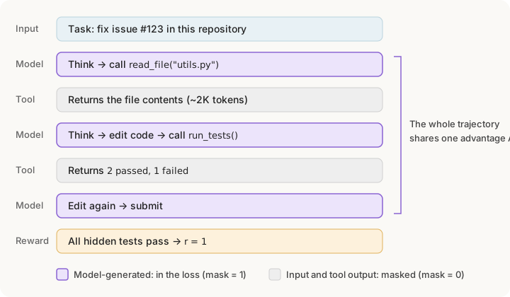
The good news is that the algorithm barely changes. It’s still rollout, score, group advantage, clipped update. What changes is everything around it:
-
The environment is now real. In LLM RL, the “environment” just appended a token. Now it runs code and returns results that can be slow, unpredictable, or have side effects (a command might delete a file). Each rollout needs its own isolated sandbox, such as a Docker container, and training may run hundreds or thousands of them at once. Building this infrastructure is often harder than the algorithm itself.
-
Loss mask. The text a tool returns was not written by the model, so it isn’t one of the model’s actions. It would make no sense to “make the tool’s output more likely”, so we don’t compute a \(\log\pi\) gradient on those tokens. Only the tokens the model wrote (the purple parts in the figure) are used in the update. The rest are masked out.
-
Credit assignment is harder. The task might take 30 steps before we know whether it succeeded. Which of those 30 steps made the difference? This is the credit assignment problem. The most common approach is still the simple one: plain GRPO at the trajectory level, where every step shares one \(A\). Ideas for doing better include giving intermediate rewards for each round, or branching several trajectories from a middle step and comparing how the branches end up.
-
The q problem gets worse. Some trajectories finish in 3 steps; others take 50. If training waits for the slowest one, most GPUs sit idle. So rollouts are usually run asynchronously: the model keeps updating while older rollouts are still coming in. That means some trajectories were generated by a version of the model that is several updates old. In our language, \(q\) is now further from \(p\), and the importance sampling corrections and caps from Sections 6 and 7 matter even more.
-
Long context. A single trajectory can run to tens or hundreds of thousands of tokens. If the system truncates or summarizes the context during rollouts, training must see exactly the same truncated or summarized version. Otherwise the states used for training don’t match the states the model actually acted in, which is yet another mismatch between \(q\) and \(p\).
-
Reward hacking. Models are very good at finding loopholes. A coding agent rewarded for passing tests might learn to edit the tests, or to hard-code the expected output. Reward design and sandbox isolation have to plan for this from the start.
-
Task data. You need lots of tasks that can be checked automatically and have the right difficulty: real GitHub issues with hidden tests, or multi-step search questions with known answers. The difficulty filter works for the same reason as in Section 7. Tasks that are always solved, or never solved, give no gradient.
Two typical examples:
- Coding agent: given a code repository and an issue, the model reads files, edits code, and runs commands, over and over. Hidden tests decide whether it succeeded.
- Search agent: the model searches several times, reads the results, and gives a final answer. It gets the reward if the answer matches the reference.
Summary: one set of symbols all the way through
Here is the whole post in one table. Read each row from left to right and notice how little the ideas change.
| Dice | Classic RL | LLM RL | Agentic RL | |
|---|---|---|---|---|
| \(p\) (what we care about) | The loaded die | Trajectories from the current policy | Responses from the current model | Multi-turn trajectories from the current model and its tools |
| \(f\) (the score) | Payout | Return | Reward for the response | Whether the task was completed |
| \(q\) (what we actually sample from) | The fair die in your hand | The old policy | The inference engine’s copy of the model | A model several updates behind, due to asynchrony |
| One sample | One roll | One trajectory | One response | One full attempt at the task |
| How we reduce variance | Roll more | Baseline or critic | Group average (GRPO) | Group average, plus intermediate rewards or branching |
The two conditions from Section 2 never went away:
- We need samples from \(p\), but in practice we almost always get them from a slightly different \(q\). Importance ratios, PPO’s clip, and TIS are all ways to correct for that, and they matter more the further right you go in the table.
- The variance must stay small. Baselines, critics, group averages, and difficulty filtering are all ways to get a clean learning signal out of noisy rewards.
Once you see these two problems, most of the new methods in LLM and agentic RL become easier to place. For each one, it’s worth asking: which of the two is it trying to fix?
References
- Williams, Ronald J. “Simple Statistical Gradient-Following Algorithms for Connectionist Reinforcement Learning.” Machine Learning 8, 1992.
- Schulman, John, et al. “High-Dimensional Continuous Control Using Generalized Advantage Estimation.” arXiv:1506.02438, 2015.
- Schulman, John, et al. “Proximal Policy Optimization Algorithms.” arXiv:1707.06347, 2017.
- Ouyang, Long, et al. “Training Language Models to Follow Instructions with Human Feedback.” NeurIPS, 2022.
- Shao, Zhihong, et al. “DeepSeekMath: Pushing the Limits of Mathematical Reasoning in Open Language Models.” arXiv:2402.03300, 2024.
- Ahmadian, Arash, et al. “Back to Basics: Revisiting REINFORCE Style Optimization for Learning from Human Feedback in LLMs.” ACL, 2024.
- Lambert, Nathan, et al. “Tülu 3: Pushing Frontiers in Open Language Model Post-Training.” arXiv:2411.15124, 2024.
- Yu, Qiying, et al. “DAPO: An Open-Source LLM Reinforcement Learning System at Scale.” arXiv:2503.14476, 2025.
- Yao, Feng, et al. “Your Efficient RL Framework Secretly Brings You Off-Policy RL Training.” Blog post, 2025.
Citation
Haoyan Luo. “From Dice to Agents: Reinforcement Learning in One Set of Symbols.” Haoyan's Blog (Sep 2026). https://clarenceluo78.github.io/blog/rl-from-dice-to-agents/.
@article{luo2026luo2026rldice,
  title   = "From Dice to Agents: Reinforcement Learning in One Set of Symbols",
  author  = "Luo, Haoyan",
  journal = "Haoyan's Blog",
  year    = "2026",
  month   = "Sep",
  url     = "https://clarenceluo78.github.io/blog/rl-from-dice-to-agents/"
}